Detailed Documentation
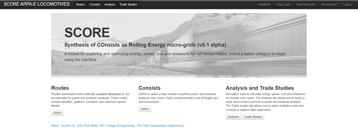
The locomotives testbed is an online analysis framework that calculates the fuel consumption and emissions of consist over a route, to access the impact different locomotive technologies have across a rail network system with various freight requirements. The locomotives testbed is partitioned into four main categories:
• Routes: a list of prepopulated routes, including gradient and curvative metrics.
• Consists: a list of consists with locomotives and freight cars, where users can develop custom consist configurations
• Analysis: Performs a fuel and emissions analysis for a selected Route and Consist
• Trade Studies: Performs a trade study with multiple Routes and Consists
Route Data
The route data is based on geolocation track information from the NARN Database. The elevation of the track is queried using the USGS web service, which allows users to query elevations for a given latitude and longitude. Once all track elevations are queried, the elevation is smoothed, since the queried elevations include noise, such as tunnels, bridges, and urban buildings. The following is a list of steps for the route generation.Download route paths (list of latitude and longitude positions) Route data is available from the NARN Database
Query elevation data for each position USGS Elevation Service
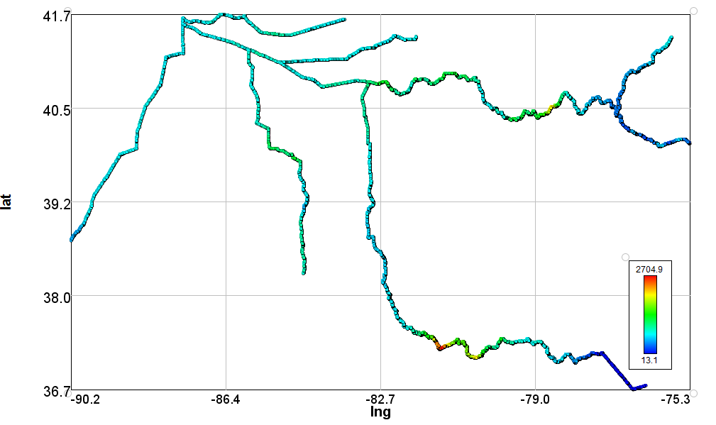
Below is code used to query the USGS elevation database and the below image displays elevation (ft) results for a queried set of routes
api_url = "https://nationalmap.gov/epqs/pqs.php?x="+str(lng)+"&y="+str(lat)+"&units=feet&output=json"
response = requests.get(api_url)
elev = float(response.json()['USGS_Elevation_Point_Query_Service']['Elevation_Query']['Elevation'])
Append latitude and longitude with Cartesian coordinate (x,y) positions
x = (np.radians(lng) - np.radians(mean_lng))*6378137.0*math.cos(np.radians(lat)) y = (np.radians(lat) - np.radians(mean_lat))*6378137.0
Select a route starting point, and order route locations based on minimum distance from previous location using Euclidean distance
dist = math.sqrt((x1 - x2)**2 + (y1 - y2)**2)
Filter small route segments based on segment_length < MIN_TOLERANCE
Calculate the radius of curvature for each route segment

Calculate degree curvature per 100 ft chord
degCur_100ft = (180/math.pi)*2*np.arcsin(50/radius)
Apply a smoothing filter on elevation data to reduce noise effects of bridges, tunnels, and buildings. scipy.signal.savgol_filter(d_elevs, WINDOW_SIZE, 3)
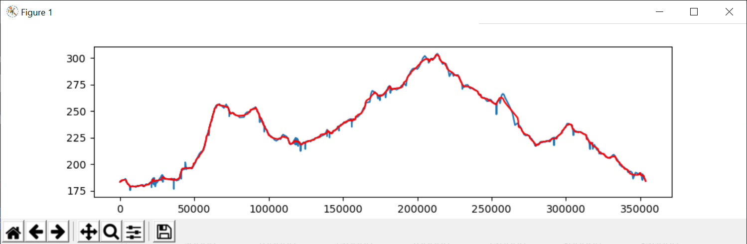
Calculate gradient of each line segment using smoothed elevation data and arc lengths
if |gradient| > 2%, assign clipped gradient and include delta elevation to the next segment.
segment_gradient = 100*(Δelev)/(track_segment_length)
Once route are generated, they are loaded into the testbed. The Routes view shows all loaded routes, as shown in the below image.
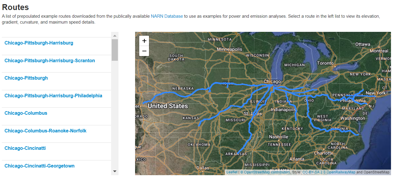
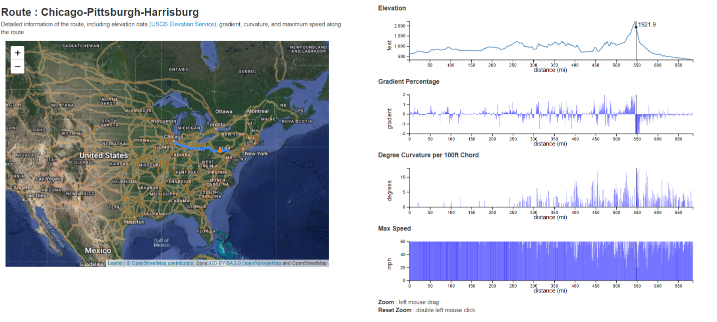
To view the details of a route, select a route link to view its details, which include elevation, gradient, curvature, and maximum speed values. One can highlight the location within the plots views, and a geolocation point identifies its position in the map view. When one zooms within the plots view, the map view is updated with the queried section of track. Zoom operations are performed using the left mouse button and drag controls.
Consist Data
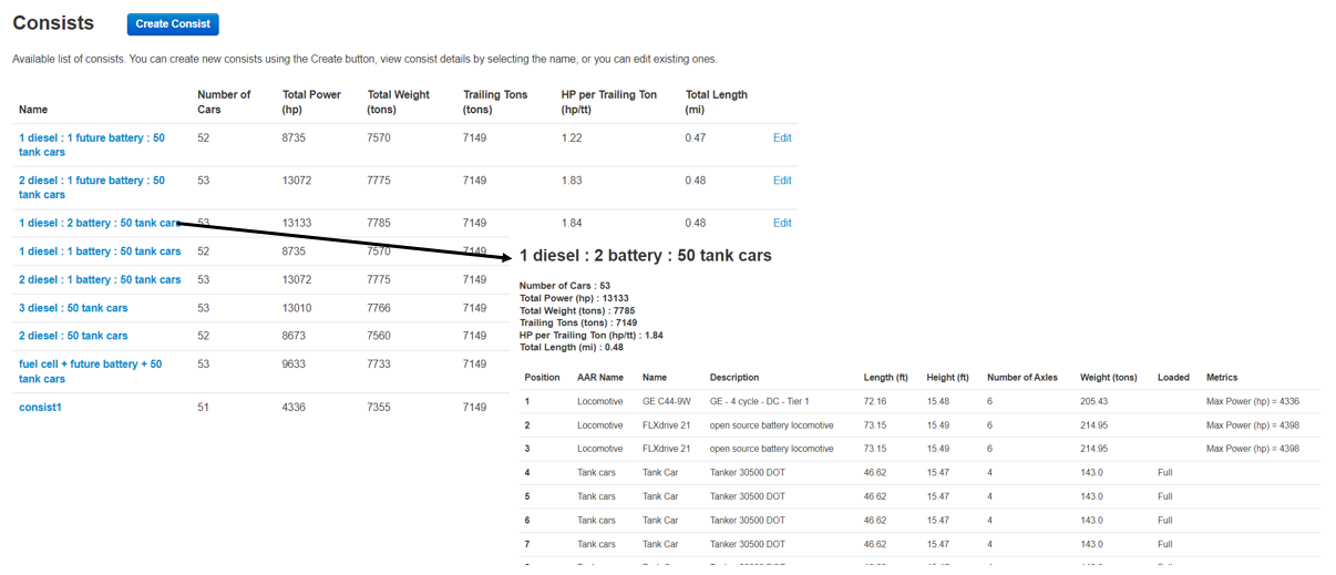
The below image shows a list of prepopulated consists, where each consist has a link to open and view its details. In the detailed view, all cars of the consist are listed in a table view, where the first car is the first row of the table. The table includes dimensions of the car, weight, and overall power capabilities if it is a locomotive.
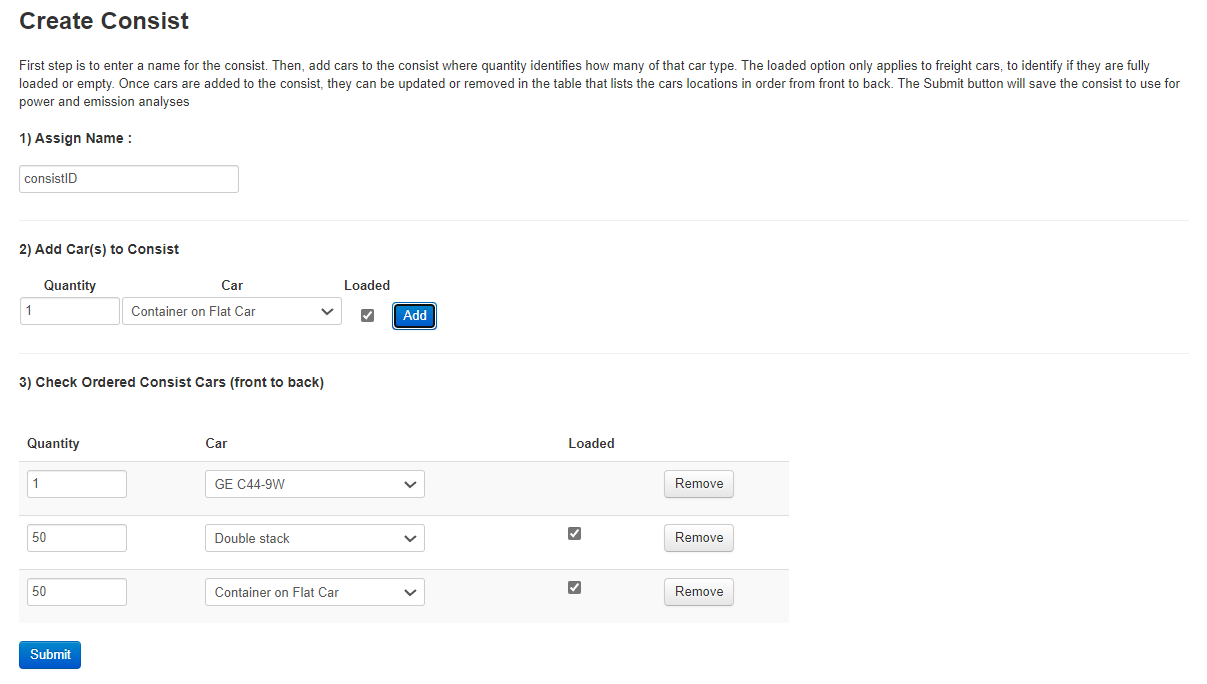
The interface to create and edit a Consist is shown below. Users assign a name to the consist, and then they add cars to the consist. When adding cars, on can choose from the following options
• Container on Flat Car
• Double Stack
• Tank Car
• Trailer on Car
• Diesel/Battery/Electric/Hydrogen Locatives
The below shows a list of prepopulated Diesel, Battery/Electric, and Fuel Cell locomotives.
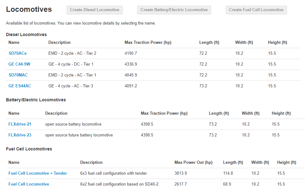
One can select links to open the details of the locomotives. For Diesel locomotives, the user can view power, dimension, and fuel properties, along with power and emissions/fuel curves for the locomotive.

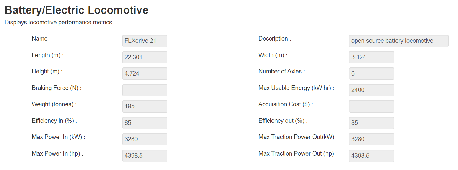
For battery/electric locomotives, the user can view power, dimension, and energy properties.
Analysis
The energy Linear Train Dynamics (eLTD) model calculates the energy flows required to move a consist along a route following a powering policy. Energy flows from stored sources such as diesel fuel, batteries, and hydrogen. This stored energy is converted to mechanical power with levels of efficiency and maximum rates given by the chosen technologies. This power passes through transmissions to eventually apply force to track with the locomotive drive wheels. The energy stored in diesel and hydrogen can only be consumed. The energy stored in the batteries can be either consumed or regenerated through braking.
GUI Frontend
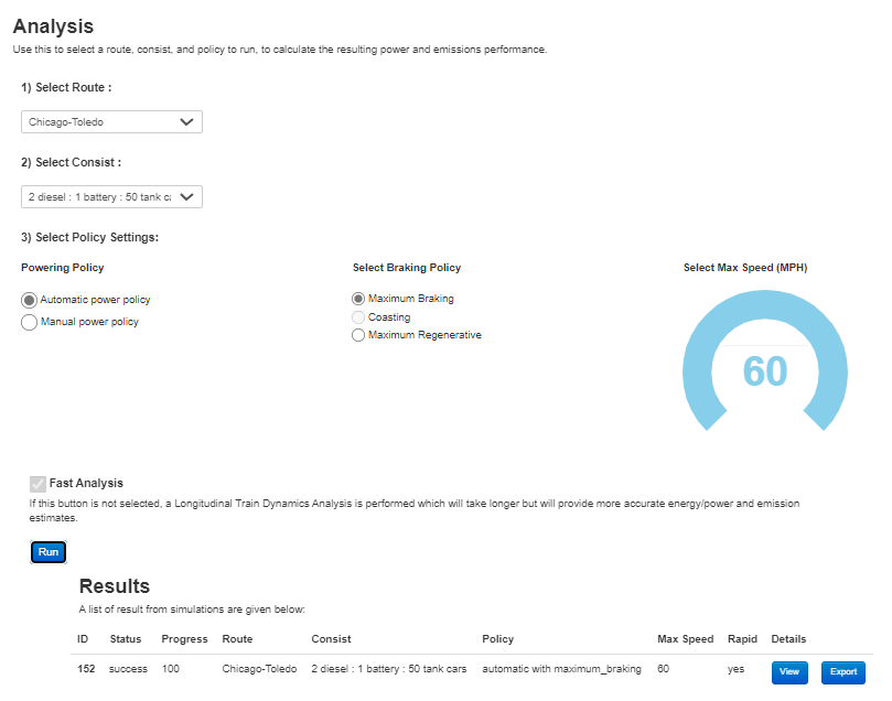
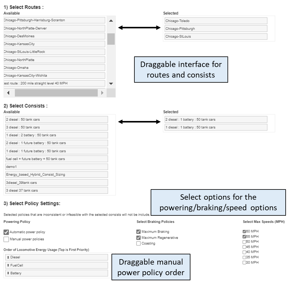
The below image displays the interface to enter the route, consist, powering policy, braking policy, and maximum speed setting for the analysis. The user selects a route and consist included in the preloaded route and consist views. The user then selects the powering policy and braking policy, where the details of each policy are described in the next section. The maximum speed of the consist is set using the radial control. Selecting the Run button will send a perform analysis message to the server, where it will place the analysis in a queue and perform an ELTD algorithm analysis on the server and return results. Once results are returned, the View and Export buttons will become enabled. Selecting the View Button will open the results view.
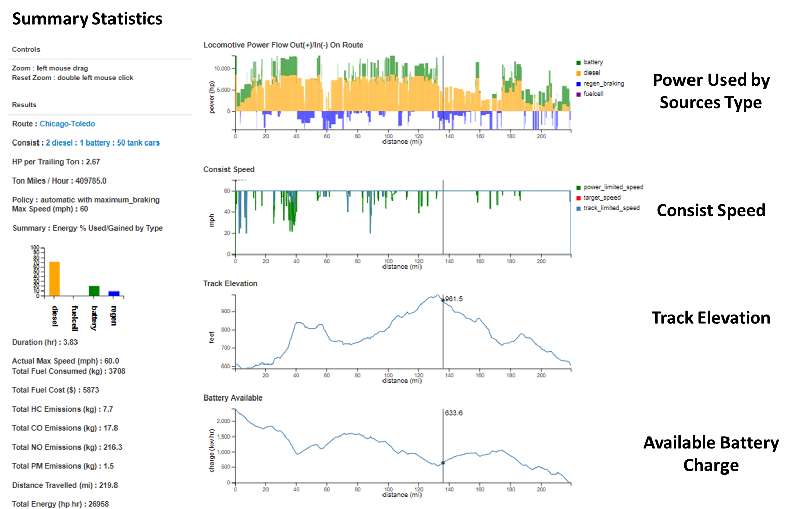
The below figure displays the results of an ELTD analysis results within the SCORE framework. The left side of the Results page shows a summary of the analysis. The following variables are included in the left side of the panel.
• Duration_hrs : total duration to travel the route without stops
• Diesel_consumed_kg : total diesel consumed by the consist in kilograms
• Hydrogen_consumed_kg : total hydrogen consumed by the consist in kilograms
• Energy_cost : estimation of diesel and hydrogen cost
• Cost_per_ton_mile : proportion of energy cost based on moving a ton of freight per mile
• Max_speed_mph : the maximum consist speed in miles per hour
• Power_order : order of using locomotive power sources based on energy required
• Braking : braking policy of the consist
• Total_weight_tons : the total weight of the consist in tons
• Number_of_cars : the total number of locomotives and freight cars included in the consist
• Trailing_weight_tons : the total weight of the freight cars in the consist
• Max_power_hp : the maximum power of a diesel or fuel cell locomotive in horsepower
• Max_battery_energy_kw_hr : the maximum power of the battery/electric locomotive in kilowatt hours
The right side of the Results Page shows a set of four plots, where the top plot shows the power used along the route based on source type. In this plot, yellow, green, and blue represent diesel, battery/electric, and regenerative power used along portions of the route. The below graph shows the consist speed, where blue represents the track maximum allowable speed, and the green represents the power limited consist speed as a result of the ELTD analysis. The track elevation is displayed in the following line plot, and the last plot shows the available battery/electric charge in the consist.
Algorithm Description
The total energy in the system is calculated using one of two appraoches. The first is a time-step integration that is more accurate but more computationally expensive. The second method is integration over distance that is less accurate but more computationally efficient.
The following summarize key algorithm approaches:
1. The route is divided into short (in most cases 100 meters or less) intervals.
2. The drag coefficients for all car elements in the consist are combined to calculate drag as a function of speed using the Canadian National resistance model.
3. The track resistance for a consist is calculated a function of consist position (first car – locomotive) along the route.
4. The maximum allowable speed is calculated as a function of track conditions (degree curvature rules).
The targets speeds along a route are calculated using a two step process. In first step, the target speed for each segment is set to either the maximum speed permitted by the track conditions or a maximum speed set by the powering policy. A second step is then used to reduce target speed due to limitations in braking, prior to portions of the track that require reductions in the maximum allowable speed. The target speed also needs to consider segments where the gradient is providing more power than the brakes can manage to maintain maximum speed. Air brakes are used for this situation to maintain any maximum speed limits. The external forces for the current interval are determined, including the track drag as a function of position, the aerodynamic drag as a function speed (taken as the final target speed) and the forces from the track gradient. The maximum allowable braking force is then added to these forces. From this sum of forces and the total mass of the consist, the acceleration (in most cases a deceleration) is calculated for the interval. The target speed for the interval can then be set given the target speed for the next interval and the acceleration. This iterative process will keep moving back the route until the target speed for the interval is greater than or equal the maximum allowable speed.
The first difference between the two integration techniques occurs when determining the target speeds for slowing a consist safely. For the distance integration, the external forces for the current interval are determined. These include the track drag as a function of position, the aerodynamic drag as a function speed (taken as the final target speed) and the forces from the track gradient. The maximum allowable braking force is then added to these forces. From this sum of forces and the total mass of the consist, the acceleration (in most cases a deceleration) is calculated for the interval. The target speed for the interval can then be set given the target speed for the next interval and the acceleration. This iterative process will keep moving back the route until the target speed for the interval is greater than or equal the maximum allowable speed set in the first pass.
The target speed is set for the time integration method by integrating backwards in time. Given the desired final state for each segment, the instantaneous drags or forces are calculated given the consist’s states (position and speed) and the consist moved backward in time to determine the required starting states at the beginning of the segment. The ending speed becomes the target speed for the segment.
Once the target speeds are established for the combined route and consist, the eLTD model can be evaluated. The motion of the consist has an initial state of position, speed, and acceleration (0.0 for each). Force is applied to the tracks by the drive wheels while resistance is calculated at each integration point. Resistance is a function of consist properties, track properties, and the speed of the consist. Additionally, changes in kinetic and potential energy are calculated as the consist changes speed and elevation. For the distance integration method, these forces are assumed constant across the segment.
During the simulation, a command for power or braking is set for each segment. This command is determined given the current speed and the target speed for the current segment. It is held constant throughout the segment for either evaluation method. The power command can be set to any continuous value between the minimum and maximum values. It is not restricted to the traditional “notch level” used for locomotives.
Power Policies
A powering policy is required to evaluate the energy flow into and out of a consist following a route. In general there are two competing objectives when evaluating a powering policy, consumed energy cost and time to traverse a route. The simulation includes two categories for a powering policy: manual and automatic. The manual policy is an a priori policy that makes decisions on power distribution based on current states and a user-defined power policy order. The automatic powering policy minimizes energy cost while still minimizing time to traverse a route. Given the total power levels for each segment, a naive strategy is taken to always push any excess diesel or hydrogen energy back into the battery in addition to regenerative braking. There are often situations where there is still insufficient battery energy to power the consist at the given maximum speed. This will often occur going up long gradients. If there is insufficient stored battery energy, then the maximum speed is reduced until this constraint can be satisfied. Once the maximum speed has been updated, a constrained linear optimization problem is solved to minimize energy cost for the route. The optimization problem determines the optimal allocation of energy sources for each segment. The dimensionality of this problem is reduced by grouping adjacent segments that have similar power requirements. A maximum size constraint is still imposed (typically not more than 10 original segments) are combined into a single larger segment used in the optimization.
Trade Studies
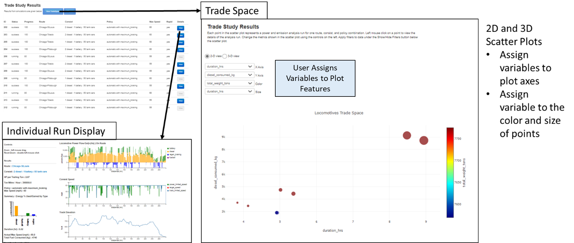
A Trade Study Analysis is performed using the Trade Studies link in the top toolbar or button on the main page. This will open a trade study input page, where a user selects multiple routes, consists, powering policies, braking policies, and maximum consist speeds. For each combination of inputs, a ELTD analysis will run on the server, and results for each run are listed in the Trade Study List at the bottom of the input page.
The below shows the resulting Trade Space Results list, where users select the TradeSpace button to explore all runs combined into scatter plot views or select the View button for each run to load the individual results view, as discussed in the previous section. For the Trade Space Exploration View, users have the ability to assign ELTD variables of interest to plot features, including spatial position, size, and color of points.