Quick Start

The locomotives testbed is partitioned into four main categories:
• Routes: a list of prepopulated routes, including gradient and curvative metrics.
• Consists: a list of available consists, with locomotives and freight cars, where users can develop custom consist configurations
• Analysis: Performs a fuel and emissions analysis for a selected Route and Consist
• Trade Studies: Performs a trade study with multiple Routes and Consists

Routes

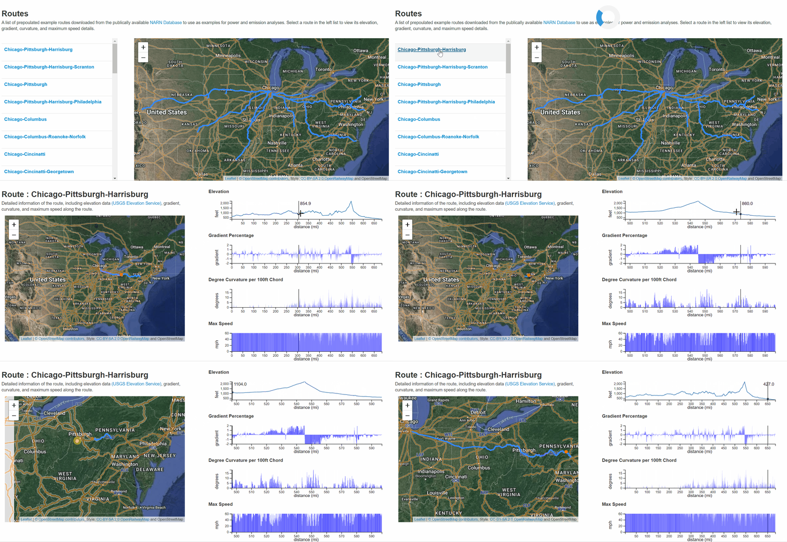
A list of prepopulated routes is displayed using the Routes link in the top toolbar or button on the main page. To view the details of a route, select a route link to view the individual route, which displays elevation, gradient, curvature, and maximum speed values. One can highlight the location within the plot views, and a geolocation point identifies its position in the map view. When one zooms within the route plots, the map view is updated with the queried section of track. Zoom operations are performed using the left mouse button and drag controls.

Consists

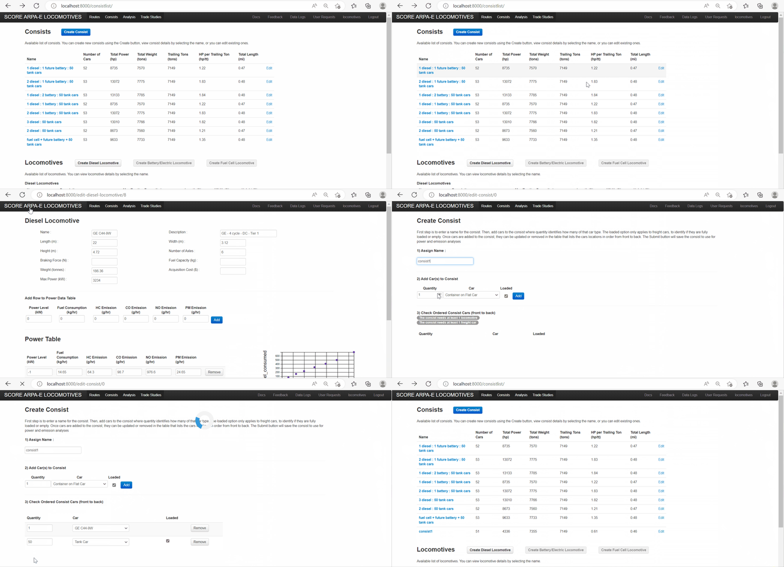
A list of prepopulated consists is displayed using the Consists link in the top toolbar or button on the main page, along with a list of predefined diesel, battery/electric, and fuel cell locomotives. Users can view the details of consist and locomotives by selecting the name links, and a new window will show the details of the selected consist car. Users can create custom consist configurations using the Create Consist Button, where each consist can include [1,N] cars, where there needs to be at least one locomotive to drive the consist. The user can assign an identifier or name to the consist, and they can add cars to the consist. When adding cars, on can choose from the following options : Container on Flat Car , Double Stack , Tank Car , Trailer on Car , Diesel/Battery/Electric/FuelCell Locatives

Analysis

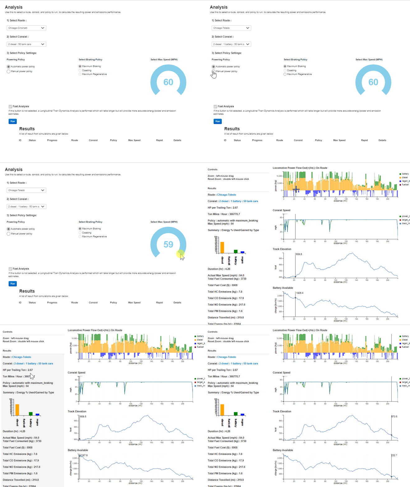
A fuel and emissions analysis is performed using the Analysis link in the top toolbar or button on the main page. This will open an analysis input page, where a user enters the selected route, consist, powering policy, braking policy, and maximum consist speed. All analyses are sent to the server and results are returned to the Results list. Selecting the View button opens a results view, where power usage is partitioned by type along the distance of a route, along with speed, track elevation, and battery usage using bar/line graphs on the right of the view (where the x axis represents the distance along the route). Summary metrics are displayed on the left of the Results display. A description of variables is as follows:
• Duration_hrs : total duration to travel the route without stops
• Diesel_consumed_kg : total diesel consumed by the consist in kilograms
• Hydrogen_consumed_kg : total hydrogen consumed by the consist in kilograms
• Energy_cost : estimation of diesel and hydrogen cost
• Cost_per_ton_mile : proportion of energy cost based on moving a ton of freight per mile
• Max_speed_mph : the maximum consist speed in miles per hour
• Power_order : order of using locomotive power sources based on energy required
• Braking : braking policy of the consist
• Total_weight_tons : the total weight of the consist in tons
• Number_of_cars : the total number of locomotives and freight cars included in the consist
• Trailing_weight_tons : the total weight of the freight cars in the consist
• Max_power_hp : the maximum power of a diesel or fuel cell locomotive in horsepower
• Max_battery_energy_kw_hr : the maximum power of the battery/electric locomotive in kilowatt hours

Trade Studies

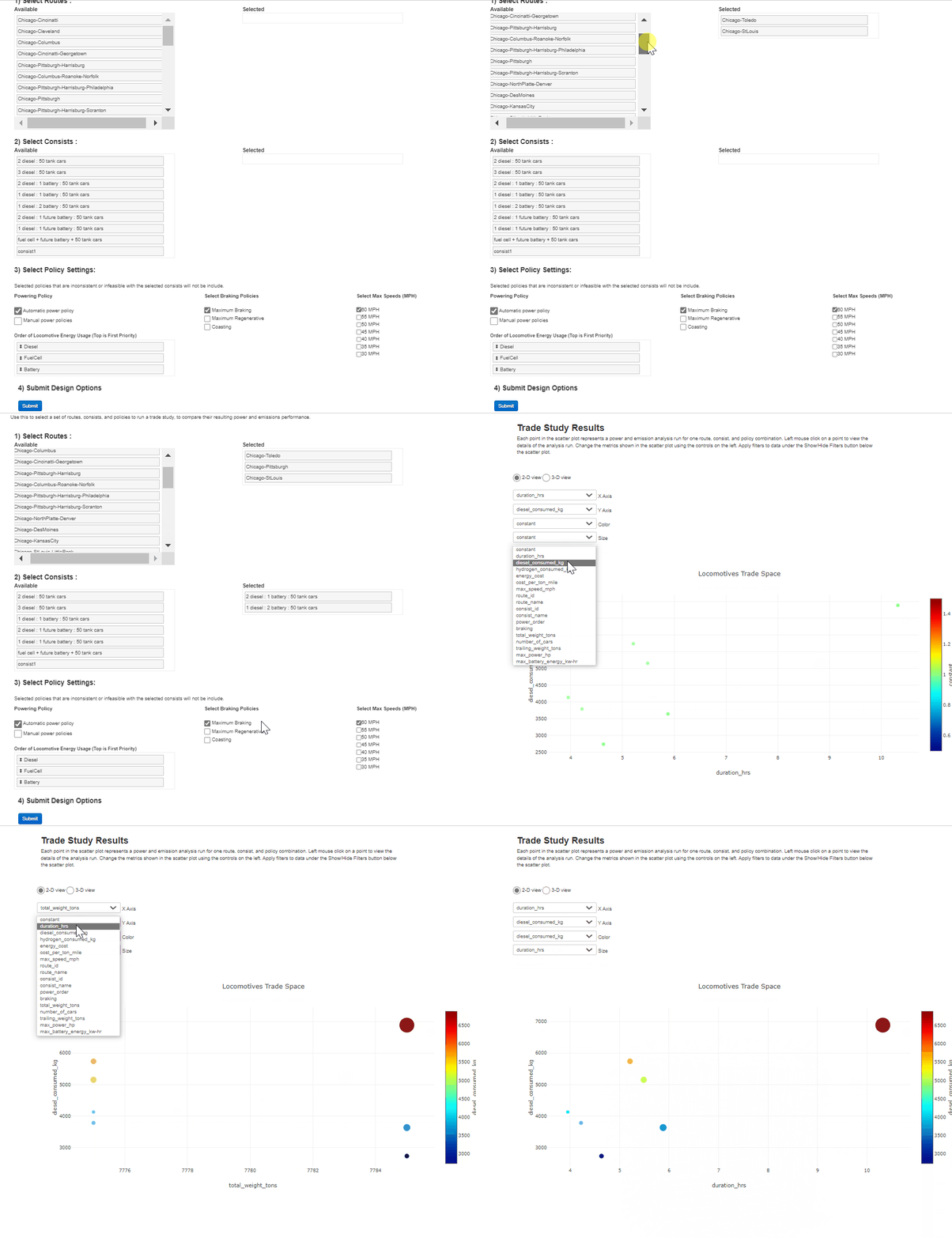
A Trade Study Analysis is performed using the Trade Studies link in the top toolbar or button on the main page. This will open an trade study input page, where a user selects multiple routes, consists, powering policies, braking policies, and maximum consist speeds. For each combination of inputs, a ELTD analysis will run on the server, and results for each run are listed in the Trade Study List at the bottom of the input page. The View TradeSpace Button opens a new window, where all runs are included within either a 2D or 3D scatter plot as a point. Users can place any variable on the spatial axes of the plot, along with assigning variables to the color and size of points.